
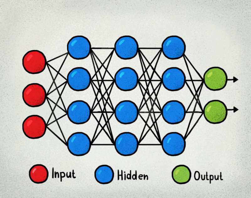
Designing a neural network means creating the right architecture to achieve optimum results. This optimum, more than often, is 'vague' as this depends on the balance of model performance and computational expenses required to train the model and predict. However, even with this loosely defined term 'optimum', to begin with any kind of neural network, you would need to come up with a starting point. In sequential models involving multilayer perceptrons (MLP), one of the key starting point is the number of hidden layers and the number of nodes required for these layers. In the absence of other data, such as the loss function required, this question can become even trickier.
Therefore, below I present a method which if used properly should provide at least an estimate of the numbers closer to actual optimum number for these parameters. As you may well be aware that the scikit-learn library of Python provides us with a GridSearchCV algorithm to tune models created with the scikit-learn library. Scikit-learn also provides methods to create neural networks. However, for creating neural network models, the scikit-learn methods are not popular. The reason for this is that there are more specialized libraries such as TensorFlow and Keras to design neural networks. Models created with other libraries are not compatiable with scikit-learn's GridSearchCV.
To overcome this difficulty, luckily Keras developers have provided a method of transforming Keras models as scikit-learn models by wrapping them with the KerasClassifier or KerasRegressor class. We are going to use this approach to first transform our Keras models into scikit-learn models and then use the GridSearchCV method to estimate the optimum number of hidden layers and number of nodes for these layers.
To begin with, we are going to use the diabetes dataset which we used in our previous post and then build a Sequential neural network to predict whether a patient is diabetic or not.
We first import the necessary functions and libraries. Note that, if you do not have some of these libraries (such as TensorFlow or Sklearn) in your Python environment, then you would need to install them beforehand.
import pandas as pd
import math

from tensorflow.keras.models import Sequential
from tensorflow.keras.layers import Dense

from tensorflow.keras.wrappers.scikit_learn import KerasClassifier

from sklearn.preprocessing import MinMaxScaler
from sklearn.model_selection import train_test_split

from sklearn.model_selection import GridSearchCV, RandomizedSearchCV
As you can see that above, we have imported the required Keras models and layers from Google's TensorFlow module. You can also install the simple Keras module instead of the TensorFlow module as per your requirement. Also note that we imported the KerasClassifier which allows us to wrap Keras models into scikit_learn models. Further, we also imported the GridSearchCV method.
Next we read the diabetes dataset and create the data-frames for the feature matrix (X) and the response vector (y).
names = ['preg', 'plas', 'pres', 'skin', 'test', 'mass', 'pedi', 'age', 'class']
df_diabetes = pd.read_csv('diabetes.csv', names = names)

df_diabetes.head() #To visually inspect the dataframe
X = df_diabetes[['preg', 'plas', 'pres', 'skin', 'test', 'mass', 'pedi', 'age']]
y = df_diabetes['class']
We would need to normalize the input features so that they are on the same scale (between 0 and 1). This is so that the errors calculated for back-propagation, while training our neural network weights, are calculated from a similar scale of features. This would mean smaller initial errors compared to that from non-normalized feature data. Smaller scale of errors leads to faster convergence of the gradient descent when adjusting the weights using the chosen cost function. To normalize we use the MinMaxScaler. You may also use the StandardScaler for the same purpose.
scaler = MinMaxScaler(feature_range=[0, 1])
X_rescaled = scaler.fit_transform(X)
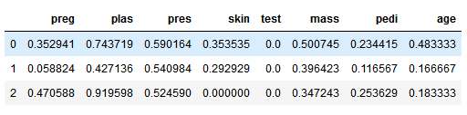
X = pd.DataFrame(data = X_rescaled, columns = ['preg', 'plas', 'pres', 'skin', 'test', 'mass', 'pedi', 'age'])
X.head(3)
This is how our normalised features would look like. See that all our features have values between 0 and 1.
Next we convert our feature matrix (X) and response vector (y) to numpy matrix and vectors. This is a method from the new pandas library.
X= X.to_numpy()
y = y.to_numpy()
Function to vary number of nodes
Now we define a custom function to generate the number of nodes for the hidden layers, by linearly varying the number of nodes between the supplied values for the outermost hidden layers.
def FindLayerNodesLinear(n_layers, first_layer_nodes, last_layer_nodes):
    layers = []

    nodes_increment = (last_layer_nodes - first_layer_nodes)/ (n_layers-1)
    nodes = first_layer_nodes
    for i in range(1, n_layers+1):
        layers.append(math.ceil(nodes))
        nodes = nodes + nodes_increment

    return layers
To demonstrate how this function works see the outputs below. Say we have 5 hidden layers, and the outermost layers have 50 nodes and 10 nodes respectively. Then the middle 3 layers should have 40, 30, and 20 nodes respectively, if we want a linear decrease in the number of nodes.
FindLayerNodesLinear(5, 50, 10)
# Output
# [50, 40, 30, 20, 10]
It is also possible to keep the number of nodes constant (by keeping the number of nodes for the outermost layers equal). With this function, it is also possible to increase the number of nodes by keeping the number of nodes for the left outer hidden layer less than that of the right outer hidden layer, however, this is not advised.
Function to dynamically change model parameters
Next, we create a function which would allow us to vary the parameters of a tensor flow model by dynamically creating a new model based on given parameters.
def createmodel(n_layers, first_layer_nodes, last_layer_nodes, activation_func, loss_func):
    model = Sequential()
    n_nodes = FindLayerNodesLinear(n_layers, first_layer_nodes, last_layer_nodes)
    for i in range(1, n_layers):
        if i==1:
            model.add(Dense(first_layer_nodes, input_dim=X_train.shape[1], activation=activation_func))
        else:
            model.add(Dense(n_nodes[i-1], activation=activation_func))

    #Finally, the output layer should have a single node in binary classification
    model.add(Dense(1, activation=activation_func))
    model.compile(optimizer='adam', loss=loss_func, metrics = ["accuracy"]) #note: metrics could also be 'mse'

    return model

##Wrap model into scikit-learn
model =  KerasClassifier(build_fn=createmodel, verbose = False)
As you could see that the above function allows us to create a sequential model of n_layers + 1 hidden layers. The number of hidden layers is n_layers+1 because we need an additional hidden layer with just one node in the end. This is because we are trying to achieve a binary classification and only one node is required in the end to predict whether a given observation feature set would lead to diabetes or not. In the function above, we provide the number of nodes in the outer hidden layers and the number of nodes for the middle layers is decided by the FindLayerNodesLinear() function as before. The activation function and loss functions provided as arguments in the function are set up for every layer. You may further customize this function to use a different activation function for every layer (such as list of activation functions of size the number of hidden layers). However, for the purpose of demonstration we are using only one activation function for all the layers. We are also using the adam Optimizer which is fast and efficient, but a different optimizer could also be used.
Define the grid for searching the optimal parameters within the grid
Now we have created the functions which allow us to change model parameters as required, we can define the grid. The grid is defined as below:
activation_funcs = ['sigmoid', 'relu', 'tanh']
loss_funcs = ['binary_crossentropy','hinge']
param_grid = dict(n_layers=[2,3], first_layer_nodes = [64,32,16], last_layer_nodes = [4],  activation_func = activation_funcs, loss_func = loss_funcs, batch_size = [100], epochs = [20,60])
grid = GridSearchCV(estimator = model, param_grid = param_grid)
As you could see that in our example, we are tuning the model to find the optimum activation and loss_functions. Note that the loss function has to be in synchronous with our model objective. Since, we are dealing with a binary classification problem, we can use either the binary_crossentropy or the hinge functions as these are well suited to binary classification models. In the grid shown above, we can find whether the optimum number of hidden layers is 2 or 3. However, you can change the n_layers to be any custom list containing the possible number of layers such as [2, 5,10,15] and the grid would allow you to find the optimum number within these possibilities. Similarly, we want to find the optimum number of nodes for our first outer hidden layer from the possible numbers 64, 32, and 16. To keep our calculations simple and fast we are keeping the number of nodes in our last outer hidden layer fixed at 4. We want to see the optimum number between 20 and 60 training epochs (i.e. the number of times the neural network is trained to find the minimum cost function).
We tune the model to find the optimum model performance and parameters by fitting the grid object with our data as below.
grid.fit(X,y)
Note that since we are using GridSearchCV, which performs cross-validation while tuning model performance we should use the entire dataset for cross-validation (i.e X and y) and not just the training-testing split training data (unless you plan to use a hold-out set). This is because in cross-validation the data is already split into training and testing sets for cross-validating with n-folds (default value in GridSearchCV is 3 fold cross-validation). Also note that since we have not provided a scoring argument to the GridSearchCV, the default 'accuracy' scoring is used to evaluate model performance while tuning.
The fitting would take some time to run. Once the grid fitting algorithm has finished running we can find the optimal model performance score (scoring metric is accuracy as explained before) and the optimal parameters as below.
Optimal Grid Parameters
print(grid.best_score_)
print(grid.best_params_)
The commands above would yield the output below.
0.7682291666666666
{'activation_func': 'relu', 'batch_size': 100, 'epochs': 60, 'first_layer_nodes': 64, 'last_layer_nodes': 4, 'loss_func': 'binary_crossentropy', 'n_layers': 3}
We see that the optimal number of layers is 3; optimal number of nodes for our first hidden layer is 64 and for the last is 4 (as this was fixed); the optimal activation function is 'relu' and the loss function is binary_crossentropy. Also the optimal number of tranining epochs is 60 which is kind of expected as 20 is too low a number to reduce the overall cost of the model.
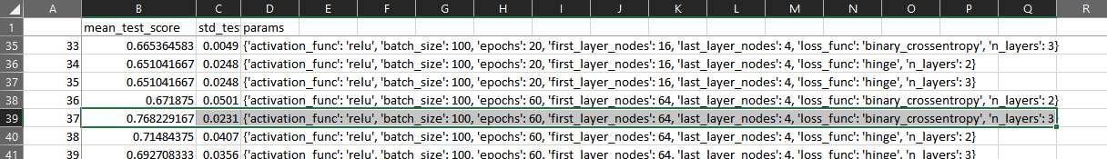
We could also see the entire model tuning operation by serialising the output as a .csv file as below.
pd.DataFrame(grid.cv_results_)[['mean_test_score', 'std_test_score', 'params']].to_csv('GridOptimization.csv')
Opening the saved csv file you could see how the grid search algorithm found the best parameters to find the maximize the accuracy.
All files used for this article including the Jupyter notebook are here.
Hope you found the article useful.
Post your comment