
In this article, we would first cover the traditional TF-IDF approach for document classification. TF-IDF stands for term frequency-inverse document frequency. TF-IDF is a numerical statistic often used as a weighing factor for words in a document, and as a proxy for how important a word in a document is in relation to all other words in a corpus containing other documents. Thereafter we would use the modern BERT approach for classifying the same documents. We would fine-tune a pre-trained BERT model for this purpose.
We would use Google-Colab for running our code. However, you could also run the code locally from your machine if you wish so.
First, we ensure that the relevant python libraries are present in our python environment. For TF-IDF, we would use the 'sklearn' library and for BERT we would use the transformers library. Colab already has 'sklearn' installed, and 'pytorch' a key dependency for the 'transformers' library is already installed. However, we would still need to install the below with pip.
Install missing libraries
! pip install transformers datasets plotly nltk
TF-IDF approach
Load datasets
Next, we need to load the 20 newsgroup dataset using 'sklearn'. On Colab we could use the 'fetch_20newsgroups' method to download and load the dataset. If using locally we can also download the dataset manually and then use the 'load_files' method to load the dataset.
# For automatically downloading the dataset and loading it to memory
from sklearn.datasets import fetch_20newsgroups
data_train = fetch_20newsgroups(subset='train', categories=None, shuffle=True, random_state=42)
data_test = fetch_20newsgroups(subset='test', categories=None, shuffle=True, random_state=42)

# # For manually downloading the dataset and loading the downloaded dataset in to memory (change the paths as relevant)
# from sklearn.datasets import load_files
# data_train = load_files(container_path=r'D:\Projects\datasets\20news\20news-bydate-train', encoding='latin', shuffle=True, random_state=42)
# data_test = load_files(container_path=r'D:\Projects\datasets\20news\20news-bydate-test', encoding='latin', shuffle=True, random_state=42)
We can inspect the loaded datasets as below.
# Inspect dataset contents
print(data_train.keys())
print(data_test.keys())

# Output
# dict_keys(['data', 'filenames', 'target_names', 'target', 'DESCR'])
# dict_keys(['data', 'filenames', 'target_names', 'target', 'DESCR'])
You would see that both the train and test datasets consist of the data (i.e. the text documents), the filenames of these text documents, the target_names i.e. the document labels in text, and the target i.e. the document labels in numbers.
We can see the list of all the unique labels (20 in total - the dataset is aptly called 20 newsgroup dataset) as below:
# View all dataset categories
list(set(data_train['target_names']))

# Output
# ['sci.electronics',
#  'talk.politics.misc',
#  'comp.sys.mac.hardware',
#  'comp.sys.ibm.pc.hardware',
#  'talk.politics.guns',
#  'comp.windows.x',
#  'sci.med',
#  'alt.atheism',
#  'comp.os.ms-windows.misc',
#  'comp.graphics',
#  'rec.sport.hockey',
#  'sci.space',
#  'talk.religion.misc',
#  'talk.politics.mideast',
#  'sci.crypt',
#  'rec.motorcycles',
#  'rec.sport.baseball',
#  'rec.autos',
#  'misc.forsale',
#  'soc.religion.christian']
Create TF-IDF vectors of the documents
We now need to create the vector representations of all the documents in the training and test datasets using the TfidfVectorizer object from 'sklearn'. We would fit the vectorizer object with the training dataset using the fit_transform method, which would first create features based on all training documents and then transform the training samples into vector representations of these features. We could do that as below.
# Tf-idf vectorizer. Create features based on training data samples and then convert training samples into vector representations of these features.
from sklearn.feature_extraction.text import TfidfVectorizer
vectorizer = TfidfVectorizer(sublinear_tf=True, max_df=0.5, stop_words='english')
X_train = vectorizer.fit_transform(data_train.data)
After this step, the training data would be converted to a sparse array of vectors i.e. a matrix representation of the entire corpus of training documents. We can inspect the matrix as below.
print("n_samples: %d, n_features: %d" % X_train.shape)

# Output
# n_samples: 11314, n_features: 129791
If you want to visualize the features, you could do something like the below. Note that the features are a long list of words, so we are only looking at a particular slice of the features.
print(vectorizer.get_feature_names()[30000:30010])

# Output
# ['asx', 'asya', 'asylum', 'asymetrix', 'asymmetric', 'asymmetries', 'asymptotically', 'async', 'asynch', 'asynchronicity']
We can visualize the Tf-idf weights for the first sample document as below.
import numpy as np
from pprint import pprint

X_train_array = X_train.toarray()
X_train_sample1_vector = X_train_array[0]

features_array = np.array(vectorizer.get_feature_names())

relevant_features_sample1 = features_array[X_train_sample1_vector > 0]
print('Features with non-zero tf-idf weights for sample 1.')
pprint(relevant_features_sample1)

print('\n')

print('Tf-idf weights for these features for sample 1.')
relevant_weights_sample1 = X_train_sample1_vector[X_train_sample1_vector > 0]
pprint(relevant_weights_sample1)

# Output
# Features with non-zero tf-idf weights for sample 1.
# array(['15', '60s', '70s', 'addition', 'body', 'bricklin', 'brought',
#        'bumper', 'called', 'car', 'college', 'day', 'door', 'doors',
#        'early', 'engine', 'enlighten', 'funky', 'history', 'host', 'il',
#        'info', 'know', 'late', 'lerxst', 'looked', 'looking', 'mail',
#        'maryland', 'model', 'neighborhood', 'nntp', 'park', 'posting',
#        'production', 'rac3', 'really', 'rest', 'saw', 'separate', 'small',
#        'specs', 'sports', 'tellme', 'thanks', 'thing', 'umd',
#        'university', 'wam', 'wondering', 'years'], dtype='<U180')


# Tf-idf weights for these features for sample 1.
# array([0.07761318, 0.17349466, 0.1700526 , 0.11686055, 0.10682953,
#        0.20483876, 0.11464293, 0.16277056, 0.08467486, 0.24391653,
#        0.09561454, 0.08115624, 0.12274527, 0.14221568, 0.10359526,
#        0.11906511, 0.16439042, 0.19103829, 0.10224976, 0.04341232,
#        0.11993249, 0.08963448, 0.05246633, 0.11298951, 0.36712898,
#        0.11075174, 0.08467486, 0.07341243, 0.13403789, 0.10839785,
#        0.16125528, 0.04371988, 0.12149832, 0.04224856, 0.13269588,
#        0.19693883, 0.06945008, 0.10014748, 0.10372149, 0.12096469,
#        0.09223978, 0.13291429, 0.13247949, 0.21683229, 0.06754479,
#        0.07616042, 0.21982819, 0.04545303, 0.26946658, 0.10886588,
#        0.07429919])
Now we have analyzed the document vectors of the training data a little bit, we need to convert the test data documents to vectors as well. (Note, that this time around we don't want to use the fit_transform method but rather just the transform method. We need to convert the test data documents into vector representations of the training features. This is because, in the real world, we may just have the training data, we build the model with the training data and expect the model to work for some unseen test data). We could do this as below.
# Create vector of the test dataset by utilizing only the features present in training dataset)
X_test = vectorizer.transform(data_test.data)
Like before, we can analyze the test document vector matrix as below.
print("n_samples: %d, n_features: %d" % X_test.shape)

# Output
# n_samples: 7532, n_features: 129791
Before training any model on the training data, we need one more thing – the train and test labels. Perform the below.
# training and test labels
y_train, y_test = data_train.target, data_test.target
At this point, we can optionally choose to reduce the number of features. So currently we have 129, 791 features – of which a number of these features (words) such as '03ii', '03i' etc. – don't make any sense. So we can optionally choose to reduce these features for better model training efficiency. Note that the tf-idf weights for such irrelevant features are already zero, so reducing the number of features would not impact model accuracy. However, it would definitely improve the training efficiency. We arbitrarily set 50,000 as the number of features (words we want to focus on). We can select the best 50,000 features based on their chi-square association score with the target variable, using the 'sklearn' SelectKBest method as below.
from sklearn.feature_selection import SelectKBest, chi2

# mapping from integer feature name to original token string
feature_names = vectorizer.get_feature_names()

# Feature reduction with Kbest features based on chi2 score
ch2 = SelectKBest(chi2, k=50000)
X_train = ch2.fit_transform(X_train, y_train)
X_test = ch2.transform(X_test)
if feature_names:
    # keep selected feature names
    feature_names = [feature_names[i] for i
                     in ch2.get_support(indices=True)]
Building the model
For training, we choose the linear support vector machine model (SVC), and then train it with the training dataset as below. The model choice is arbitrary, for this demonstration. In an ideal situation, you should start out with a set of different models and choose the one with the best performance.
from time import time
# Training our model

from sklearn.svm import LinearSVC

clf = LinearSVC(penalty="l2", random_state=123)

t0 = time()
clf.fit(X_train, y_train)
train_time = time() - t0
print("train time: %0.3fs" % train_time)
Once the model has been trained, we can validate its accuracy as below. Note that our performance metric here is accuracy but we can choose other metrics as well, such as precision, recall, etc.
# Testing our model

from sklearn import metrics

t0 = time()
pred = clf.predict(X_test)
test_time = time() - t0
print("test time:  %0.3fs" % test_time)

score = metrics.accuracy_score(y_test, pred)
print("accuracy:   %0.3f" % score)

# Output
# test time:  0.026s
# accuracy:   0.860
So, as we could see that our model with TF-IDF did a good job here and we achieved an accuracy of 86%.
BERT approach
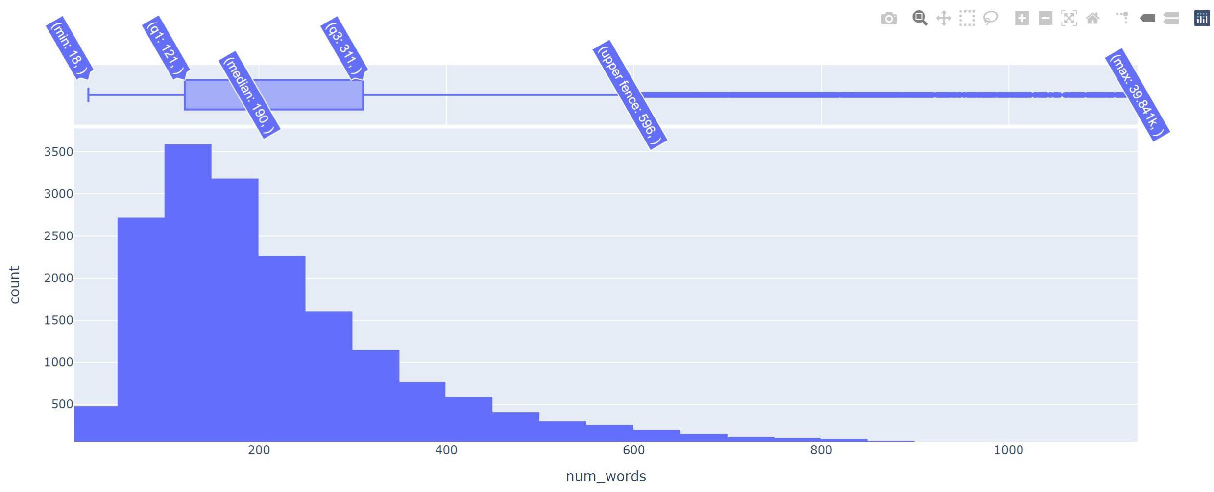
Before going any further with BERT, we need to understand that the base version of BERT has a token limit of 512 tokens. BERT converts the input text into tokens where a token is essentially a word. So, just to confirm whether our BERT model would be expected to work with our 20news group data, we can check the distribution of the number of words per document in our dataset as below. Note that the below approach is approximate as the regex tokenizer would sometimes fail to identify words, where the pattern of characters would not exactly fit the '\w+' to identify words. However, this is very close to producing the correct number of words.
# Collate all documents
docs_all = data_train['data'] + data_test['data']

# Find number of words per document in the dataset
from nltk.tokenize import RegexpTokenizer
import statistics
tokenizer = RegexpTokenizer(r'\w+')
n_words = [len(tokenizer.tokenize(doc)) for doc in docs_all]
print(min(n_words))
print(max(n_words))
print(statistics.mean(n_words))

# Output
# 18
# 39841
# 317.65207471081396
So as we could see that the minimum word count in a document is 18 and the maximum is 39,841. However, the mean is ~318 words per document. We can visualize the distribution using Plotly which we installed with pip earlier, like below.
import plotly.express as px
import pandas as pd
df = pd.DataFrame({'num_words': n_words})
fig = px.histogram(df, x="num_words", marginal="box")
fig.show()
The plot (after zooming a little bit) shows that the upper fence (q3 + 1.5 times the inter-quantile (q3-q1) range) is at 596 words per document. This means the majority of our documents have a word count of less than 596, so even if BERT caps the token count to 512 this should have little impact on our document classification task.
Pre-processing data
For working with the BERT model, we need a train, validation, and test data. We obtain these as below. We define the train and test text and labels and then split the train data further to obtain the validation data.
# Create train and test texts and labels
train_texts = data_train['data']
train_labels = data_train['target']

test_texts = data_test['data']
test_labels = data_test['target']
# Further split the train data into validation data using sklearn
from sklearn.model_selection import train_test_split
train_texts, val_texts, train_labels, val_labels = train_test_split(train_texts, train_labels, test_size=.3)
Next, we tokenize the train, test, and validation data using the original tokenizer used in the pre-trained BERT model as below.
# Tokenize the train, validation and test data
from transformers import AutoTokenizer
tokenizer = AutoTokenizer.from_pretrained("bert-base-uncased")

def tokenize_function(examples):
    return tokenizer(examples, padding="max_length", max_length=512, truncation=True)

train_encodings = tokenize_function(train_texts)
val_encodings = tokenize_function(val_texts)
test_encodings = tokenize_function(test_texts)
Please note that the above step would download the tokenizer for "bert-base-uncased" from servers of HuggingFace who are creators of the transformers library. If that was already downloaded then this step would be skipped. If you are working locally, you could also download the original pre-trained model from their website, and use the location of the downloaded model files instead of the "bert-base-uncased" instead. So you could use something like below instead.
tokenizer = AutoTokenizer.from_pretrained(r"D:\downloaded_location_of_the_model\bert-base-uncased")
We further need to transform our data to be used for the trainer API of transformers to fine-tune our BERT model with our training data.
# Transform data to be used for the trainer API of hugging face transformers
import torch

class TwentyNewsDataset(torch.utils.data.Dataset):
    def __init__(self, encodings, labels):
        self.encodings = encodings
        self.labels = labels

    def __getitem__(self, idx):
        item = {key: torch.tensor(val[idx]) for key, val in self.encodings.items()}
        item['labels'] = torch.tensor(self.labels[idx])
        return item

    def __len__(self):
        return len(self.labels)

train_dataset = TwentyNewsDataset(train_encodings, train_labels)
val_dataset = TwentyNewsDataset(val_encodings, val_labels)
test_dataset = TwentyNewsDataset(test_encodings, test_labels)
Initialize pre-trained BERT model for classification task
We now need to load the pre-trained model into memory and initialize it for a classification task with 20 labels. This can be achieved as below.
from transformers import AutoModelForSequenceClassification

model = AutoModelForSequenceClassification.from_pretrained("bert-base-uncased", num_labels=20)
You may get a message like below. This is perfectly fine.
Some weights of the model checkpoint at bert-base-uncased were not used when initializing BertForSequenceClassification: ['cls.predictions.transform.dense.bias', 'cls.predictions.transform.dense.weight', 'cls.predictions.transform.LayerNorm.bias', 'cls.predictions.decoder.weight', 'cls.predictions.bias', 'cls.seq_relationship.bias', 'cls.predictions.transform.LayerNorm.weight', 'cls.seq_relationship.weight']
- This IS expected if you are initializing BertForSequenceClassification from the checkpoint of a model trained on another task or with another architecture (e.g. initializing a BertForSequenceClassification model from a BertForPreTraining model).
- This IS NOT expected if you are initializing BertForSequenceClassification from the checkpoint of a model that you expect to be exactly identical (initializing a BertForSequenceClassification model from a BertForSequenceClassification model).
Some weights of BertForSequenceClassification were not initialized from the model checkpoint at bert-base-uncased and are newly initialized: ['classifier.weight', 'classifier.bias']
You should probably TRAIN this model on a down-stream task to be able to use it for predictions and inference.
Please note that just like the tokenizer the model can be initialized from a pre-downloaded location.
Preparing the transformers trainer API
We first create the training arguments like below.
# Create the training arguments
from transformers import TrainingArguments
training_args = TrainingArguments(evaluation_strategy="epoch",
                                  output_dir='./results',          # output directory
                                  num_train_epochs=3,              # total number of training epochs
                                  per_device_train_batch_size=8,  # batch size per device during training
                                  per_device_eval_batch_size=16,   # batch size per device for evaluation
                                  logging_dir='./logs',            # directory for storing logs
                                  logging_steps=10)
We have defined the number of epochs as 3, meaning which, our training data would be passed 3 times, during which the trainer would fine-tune the weights and biases for the entire network to minimize the training loss. The batch sizes are dependent on the GPU available, and I have chosen them depending on the GPU (Tesla K80) which was available on my Colab notebook. Batch size defines the number of training samples fed together in the model. You should not choose a very large batch size as this would reduce the accuracy of the gradient descent process (to estimate the new values of the network parameters). While a smaller batch size would be more accurate, having a too-small batch size would increase the training time.
Then we create the evaluation metric during training.
# Define the evaluation metric during training
import numpy as np
from datasets import load_metric
from sklearn.metrics import accuracy_score

def compute_metrics(eval_pred):
    logits, labels = eval_pred
    predictions = np.argmax(logits, axis=-1)
    accuracy = accuracy_score(labels, predictions)

    return {'accuracy': accuracy,}
The trainer is then defined as below.
# Create the trainer
from transformers import Trainer
trainer = Trainer(
    model=model,
    args=training_args,
    train_dataset=train_dataset,
    eval_dataset=val_dataset,
    compute_metrics=compute_metrics,
)
Training the model
Once the trainer has been initialized, we can use it to train the model. Start the training process with the command below.
# train the model
trainer.train()
This would take some time to finish. It took about 1 hour 15 minutes on my Colab notebook. At the end of every epoch, you would be able to see the value of the performance metric (accuracy in our case), along with the training and validation loss. The training loss should ideally decrease after every epoch. The validation loss would initially decrease, then stabilize for some further epochs and thereafter it might start increasing. If the validation loss starts increasing steeply after a particular epoch this implies that the model has been overfitted with the training data following that particular epoch – which means that the model should only be trained for a particular number of epochs which increases accuracy but does not lead to over-fitting. In our case, the number of epochs is 3, therefore we might not be able to see this behavior as the number of epochs is already very small.
Once the training has finished, we might see results similar to below.
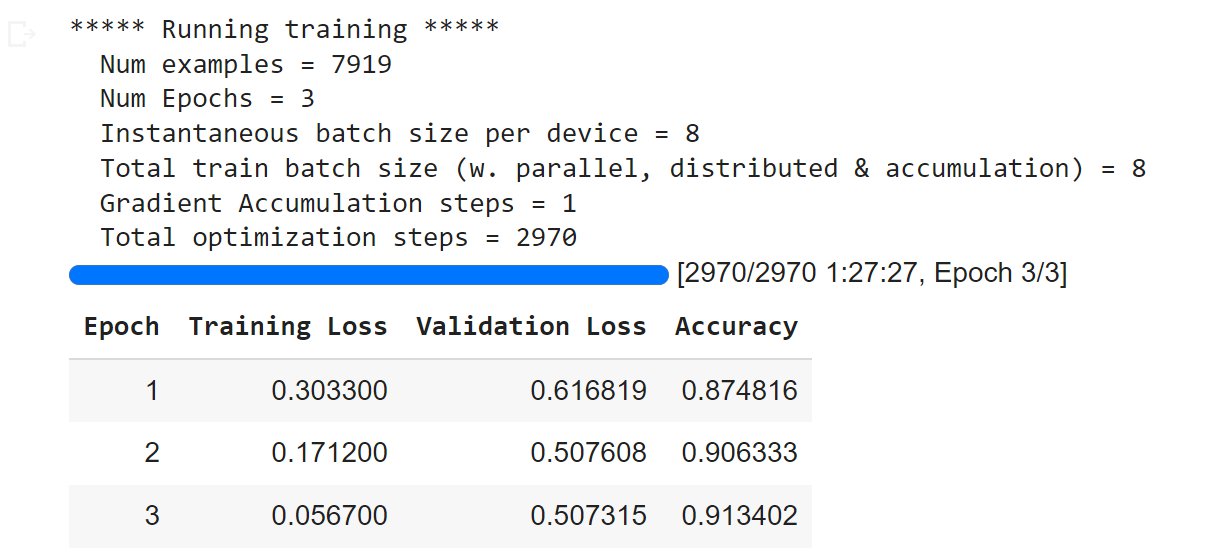
Since the validation loss has not gone up, while the training loss is going down and the training accuracy is increasing, this suggests that we might have trained for at least one more epoch.
At this point, you may want to save your model like below.
model_path = "bert-model-trained"
model.save_pretrained(model_path)
tokenizer.save_pretrained(model_path)
Now, it's time to measure the performance of our fine-tuned model on the test dataset. This can be done like below. First we define a prediction function.
# Prediction function

def get_prediction(text):
    # tokenize the input text
    inputs = tokenizer(text, padding="max_length", max_length=512, truncation=True, return_tensors="pt").to("cuda")
    # get output of the fine-tuned model for this tokenized input
    outputs = model(**inputs)
    # convert model outputs to probabilities by performing a softmax
    probs = outputs[0].softmax(1)
    # use arg max to find the index where probabilty is the maximum, this index is our predicted label for the input text
    return probs.argmax()
Next, we can use the prediction function to evaluate our testing accuracy. This can be done like below.
# Testing our model

from sklearn import metrics

t0 = time()
preds = [get_prediction(text) for text in test_texts]
pred_labels = [pred.cpu().detach().numpy().reshape(-1,)[0] for pred in preds]
test_time = time() - t0
print("test time:  %0.3fs" % test_time)

score = metrics.accuracy_score(test_labels, pred_labels)
print("accuracy:   %0.3f" % score)

# Output
# test time:  532.455s
# accuracy:   0.856
This might take some minutes to run. In my case, it took 8 minutes to run. As you could see from the output, that with a testing accuracy of 85.6%, we did not see an improvement from the testing accuracy in the case of the TF-IDF approach (86%). Perhaps, if we had trained for a few more epochs, or could have used the entire training dataset for the BERT approach, we would have achieved better results. To put it into a more positive context, the BERT model was still able to achieve almost identical performance to the TF-IDF approach with only a few epochs.
Unlike TF_IDF, the BERT models can be fine-tuned for a variety of NLP tasks and not just document classification, and the BERT models still produce results that are identical or better than traditional approaches. Further, iterations of the bi-directional transformer with attention layers, on which this particular BERT model was based, have been able to perform tasks such as question and answering, contextual similarity, next-word prediction, summarization, etc. where approaches such as TF-IDF would never work. This is because modern architectures such as BERT are able to capture the semantic meaning of words in the context of other words around them. However, approaches such as TF-IDF are still iterations of the bag-of-words approach which lays emphasis on the frequency of particular words and is unable to capture the meaning of words in the context of other words surrounding them such as that in a sentence or in a paragraph. As an example, in TF-IDF different words but with the same meaning are treated as separate words, because TF-IDF is unable to capture the relation between words.
The Colab notebook used with this article is here. Hope you liked the article and I was able to create a thought provoking hugging face 🤗 transformers moment for you. Happy transforming 🤗.
Post your comment