
To demonstrate the automated feature selection methods in Python we would use the diabetes dataset. Import the diabetes .csv file into a data-frame with Pandas as below:
import pandas as pd
names = ['preg', 'plas', 'pres', 'skin', 'test', 'mass', 'pedi', 'age', 'class']
df_diabetes = pd.read_csv('diabetes.csv', names = names)
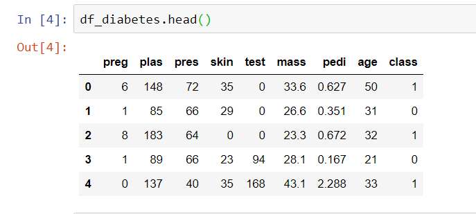
df_diabetes.head()
You should see the data frame as below:
10 of the most useful feature selection methods in Machine Learning with Python are described below, along with the code to automate all of these.
1) Remove features with low -variance
The first feature elimination method which we could use is to remove features with low variance. The thinking behind this is that features which have low variance, i.e. features which mostly remain at the same level across different observations, should not ideally be responsible for differing responses in the observations.
Select X as the set of all features, and Y as the repsonse variable. Here, the response variable Y is class.
X = df_diabetes[['preg', 'plas', 'pres', 'skin', 'test', 'mass', 'pedi', 'age']]
Y = df_diabetes['class']
We now create a VarianceThreshold object of Sklearn, with a variance threshold of 0.3 (i.e. remove features with variance less than 30%). Next we fit the VarianceThreshold object with the response variable X and the feature matrix Y.
from sklearn.feature_selection import VarianceThreshold

var = VarianceThreshold(threshold=0.3)
var = var.fit(X,Y)
With the .get_support method of sklearn classification objects we see that the feature with index 6 in the feature matrix has been eliminated.
cols = var.get_support(indices=True)
cols
#Output
array([0, 1, 2, 3, 4, 5, 7], dtype=int64)
If we now look at the feature names, we see that the feature "pedi" has been eliminated from the feature matrix.
features = X.columns[cols]
features
#Output
Index(['preg', 'plas', 'pres', 'skin', 'test', 'mass', 'age'], dtype='object')
2) Remove features which are not correlated with the response variable
For this we could use the Pearson correlation to find the features which have some degree of correlation with the response variable. It is however to be noted that although a feature may not be correlated with the response variable, it may still interact with some other variables such that the interaction of the variables helps explain the response. Strictly speaking, eliminating un-correlated variables only makes sense, if the variables are independent of all other variables. Another caveat is that one variable may show low correlation with the response, because this variable has been confounded by another variable. So, removing variables based on uni-variate correlations should only be performed, when it has been clearly proven that adding the variable doesn't have a significant improvement in model performance.
In our example, we can calculate the correlations and visualize as below. Note that we are using the matplotib and seaborn libraries for plotting the correlation matrix as a heat-map. So install these libraries beforehand:
import seaborn as sns
import matplotlib.pyplot as plt

plt.figure(figsize=(12,12))
cor = df_diabetes.corr()
sns.heatmap(cor, annot=True, cmap=plt.cm.Reds)
plt.show()
The heat map would look like below:
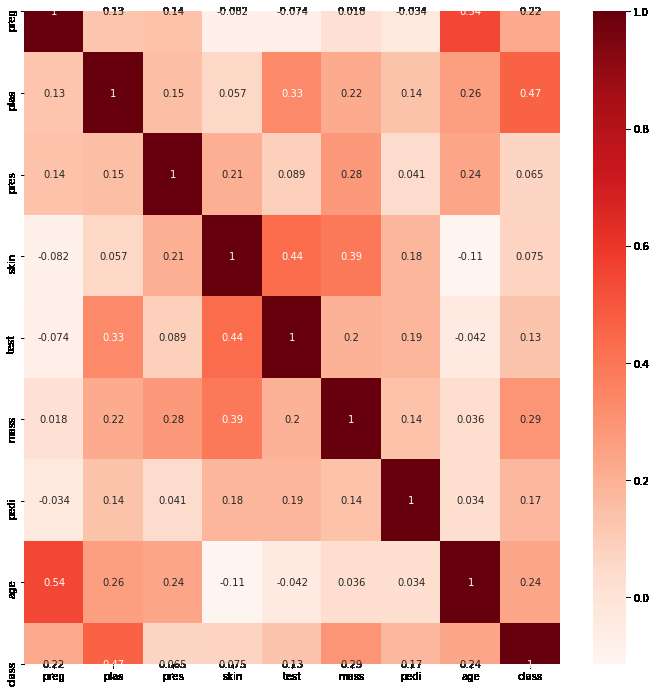
To automate this method we can create a filter to select only those features which have a correlation coefficient above a threshold (just like the variance threshold). In our case we use a threshold of 10%. The code for the filter would look like below:
# Consider correlations only with the target variable
cor_target = abs(cor['class'])

#Select correlations with a correlation above a threshold
features = cor_target[cor_target>0.1]
features
The selected features produced with the above code are shown with their correlation coefficients.
preg     0.221898
plas     0.466581
test     0.130548
mass     0.292695
pedi     0.173844
age      0.238356
class    1.000000
Name: class, dtype: float64
You can then use the features.index method to extract the selected feature column names, which you can later use on the data frame to create the feature matrix of the selected features.
features.index
#Output
Index(['preg', 'plas', 'test', 'mass', 'pedi', 'age', 'class'], dtype='object')
3) K-Best Fit
As per sklearn this method removes all but the k highest scoring features. The score is based on uni-variate statistical tests. Here, in the example below we use the ChiSquare scoring function.
As before, we first create an object of the SelectKBest class with k = 5, i.e. we want to select 5 best scoring features. The score function is chi2. Next we fit the KBest object with the response variable X and the full feature matrix Y.
from sklearn.feature_selection import SelectKBest
from sklearn.feature_selection import chi2

KBest = SelectKBest(score_func = chi2, k = 5)
KBest = KBest.fit(X,Y)
We can get the scores of all the features with the .scores_ method on the KBest object. Similarly we can get the p values. We can combine these in a dataframe called df_scores.
df_scores = pd.DataFrame({'features': X.columns, 'Chi2Score': KBest.scores_, 'pValue': KBest.pvalues_ })
df_scores
The scores look like below:
#Output

	features	Chi2Score	pValue
0	preg	111.519691	4.552610e-26
1	plas	1411.887041	5.487286e-309
2	pres	17.605373	2.718193e-05
3	skin	53.108040	3.156977e-13
4	test	2175.565273	0.000000e+00
5	mass	127.669343	1.325908e-29
6	pedi	5.392682	2.022137e-02
7	age		181.303689	2.516388e-41
Since we are interested in only 5 of the best scoring features, we can get the feature name list as below:
cols = KBest.get_support(indices=True)
cols
#Output
array([0, 1, 4, 5, 7], dtype=int64)
features = X.columns[cols]
features
#Output
Index(['preg', 'plas', 'test', 'mass', 'age'], dtype='object')
4) SelectPercentile
This is a modification to the K-Best feature selection technique where we select the top x percentile of the best scoring features. So in our example, if we say that x is 80%, we want to select the top 80 percentile of the features based on their scores.
The code is very similar to that of SelectKBest, with the only change that we provide a percentile in the SelectPercentile object created.
from sklearn.feature_selection import SelectPercentile
from sklearn.feature_selection import chi2

SPercentile = SelectPercentile(score_func = chi2, percentile=80)
SPercentile = SPercentile.fit(X,Y)
We would see that with the top 80 percentile of the best scoring features, we end up with an additional feature 'skin ' compared to the K-Best method.
cols = SPercentile.get_support(indices=True)
cols
features = X.columns[cols]
features
#Output
Index(['preg', 'plas', 'skin', 'test', 'mass', 'age'], dtype='object')
5) Sequential Feature Selectors (Step-Wise Forward Selector)
To use the sequential step wise forward feature selector we would have to use a special library called 'mlxtend'. Install this library from PyPI. As per the official package, the goal of feature selection is two-fold - to improve the computational efficiency, and, reduce the generalization error of the model by removing irrelevant features or noise. Step wise or sequential feature selectors achieve this by adding or removing one feature at a time, based on the classifier/estimator performance until a feature subset of the desired size k is reached.
Here we first use the forward selector. The code is very similar to the ones we have used above. We first create an object of the SequentialFeatureSelector class from mlextend.feature_selection. Because these feature selectors work by evaluating model performance for every added or removed feature, we need to use an estimator. Here we use the RandomForestClassfier from sklearn. Next we fit the selector object with the response variable and the feature matrix. We want to chose the best combination of 6 variables, so we set k_features = 6 in the StepForward selector object. We also want to cross-validate model performance for every combination of variables, so we provide a cv value of 5 for 5 fold cross validation. If you want to skip the cross validation, simply put a value of 0 or ignore the parameter (default value of cv is 5). For the SequentialFeatureSelector object to work as a forward selector, we set the forward value as True .
from mlxtend.feature_selection import SequentialFeatureSelector as sfs
from sklearn.ensemble import RandomForestClassifier

# Estimator
estimator = RandomForestClassifier(n_estimators=10, n_jobs=-1)
# Step Forward Feature Selector
StepForward = sfs(estimator,k_features=6,forward=True,floating=False,verbose=2,scoring='accuracy',cv=5)


StepForward.fit(X,Y)
When the above code is run, while fitting the data, it shows the best combination of features and model performance for every number of features till the k_features value is reached.
Via the .sunsets_ attribute, you can take a look at the selected feature indices at each step.
StepForward.subsets_
So you could look at the best features for each step of the iteration as below:
#Output

{1: {'feature_idx': (1,),
  'cv_scores': array([0.70779221, 0.68181818, 0.67532468, 0.7254902 , 0.76470588]),
  'avg_score': 0.7110262286732875,
  'feature_names': ('plas',)},
 2: {'feature_idx': (1, 5),
  'cv_scores': array([0.72727273, 0.67532468, 0.77272727, 0.75163399, 0.70588235]),
  'avg_score': 0.7265682030387912,
  'feature_names': ('plas', 'mass')},
 3: {'feature_idx': (0, 1, 5),
  'cv_scores': array([0.75324675, 0.67532468, 0.76623377, 0.75816993, 0.73202614]),
  'avg_score': 0.7370002546473134,
  'feature_names': ('preg', 'plas', 'mass')},
 4: {'feature_idx': (0, 1, 5, 6),
  'cv_scores': array([0.75324675, 0.7012987 , 0.74675325, 0.79084967, 0.73856209]),
  'avg_score': 0.7461420932009167,
  'feature_names': ('preg', 'plas', 'mass', 'pedi')},
 5: {'feature_idx': (0, 1, 2, 5, 6),
  'cv_scores': array([0.72727273, 0.76623377, 0.76623377, 0.80392157, 0.74509804]),
  'avg_score': 0.7617519735166794,
  'feature_names': ('preg', 'plas', 'pres', 'mass', 'pedi')},
 6: {'feature_idx': (0, 1, 2, 5, 6, 7),
  'cv_scores': array([0.73376623, 0.72077922, 0.72727273, 0.81699346, 0.73202614]),
  'avg_score': 0.7461675579322637,
  'feature_names': ('preg', 'plas', 'pres', 'mass', 'pedi', 'age')}}
You could look at the indices of the feature columns through the k_feature_idx_ method.
# Selected feature columns
cols = list(StepForward.k_feature_idx_)
cols
#Output
[0, 1, 2, 5, 6, 7]
You could use these indices to find the feature names as before.
features = X.columns[cols]
features
#Output
Index(['preg', 'plas', 'pres', 'mass', 'pedi', 'age'], dtype='object')
You could also use the inbuilt k_feature_names_ method to directly look at the feature names.
StepForward.k_feature_names_
#Output
('preg', 'plas', 'pres', 'mass', 'pedi', 'age')
Lastly you could get the best fit score of the model with the selected features, with the .k_score_ method.
StepForward.k_score_
The score in our case is below:
0.7474238180120534
6) Sequential Feature Selectors (Step-Wise Backward Selector) + Automatic best number of features
The backward method is exactly the same as above, except we start with all the features and then remove features until we find the best combination of the k_features. The advantage with this method is that if the k_number of ...
Post your comment